The Hidden Layer

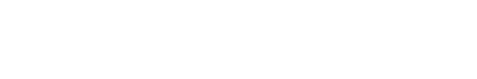
The chromosome will use 30 "nodes-in-this-layer" genes, each with a value between 0 and 1, to determine how the 75 hidden nodes will be divided among the existing hidden layers. Once it has been determined that the network will have N hidden layers (as outlined in the previous paragraph) we look at the N "nodes-in-this-layer"genes with the highest values. These N layers are the ones that will actually exist for this particular network. We then add these N "nodes-in-this-layer" real values, and use the result to compute how many nodes will be in each of these N layers with the formula

Once the number of hidden layers (and how many nodes in each of them) is determined, the connection between the layers is defined. For each layer, the chromosome has a gene that represents where it gets its input from, and another gene that represents where they send their output. Once again, we look at those N layers we have determined, as described above, that we will have. For these layers, the corresponding "get-input-from" gene stores a value between 0 and 1. By multiplying that value by N + 1 we map the "get-input-from" real value to a real value that falls between 0 and N + 1. When we round this real number to the nearest integer, we end up with an integer between 0 and N+1 that represents the number of the layer from which this particular layer takes its input. Layer #0 corresponds to the input layer. Layer # N+1 represents the output layer.

The formula for determining where a layer gets its input from is then determined by the equation

The most general of all topologies would be one where there is only one hidden layer with 75 nodes, with recursive connections to itself. In that case, we would have a total of 17475 weights. Since it is only these weights that a network can change in order to better solve a particular problem, knowledge about how to solve a problem has to be coded in the value of these weights. A network with more weights, then, has more "repositories" for this information. At the same time, being able to store too much information about the training set being presented might lead to a network that memorizes the training set, as opposed to one that finds salient properties in the data. This would lead to a network that is unable to generalize past the training data (Koncar & Guthrie, 1994 ). An approach followed by many researchers is to prune some of the weights of the network in order to find a similar network that generalizes better. Examples of this technique can be found in Solla, Le Cun & Denker, J., (1990), Stork & Hassibi (1993), Smolensky & Mozer (1989), and Dow & Sietsma (1991). All of these pruning techniques are computationally expensive, since they require retraining and retesting the network each time one or more weights are removed. By selecting a topology different than fully connected, the process outlined above reduces the total amount of connections in the network. In this way, the network is kept from having enough connections to allow it to memorize the training set. In effect, a lower number of connection forces the network to find ways to generalize, which in turn produces better performance with data outside the training set. For this reason, networks that use a high number of connections will be penalized by a factor equal to the percentage of connections they use relative to the maximum amount of connections (which is 17475). Therefore, the fitness of each network will be multiplied by (17475 - C)/17475, where C is the total number of connections it has.

The transfer function used by each hidden node will be determined by 75 additional genes. The available transfer functions will be: sign function, identity function, tangential function, step function, product function (the output of the node takes its value from the product of all weighted inputs), logistic, or no more than zero (the output turns high if the sum of weighted inputs is non-positive).

Transfer functions available to each node.

The learning function to be used to train the network will be determined by another gene. A value between 0 and .20 will indicate Backpropagation Through Time. A value between .21 and .4 will indicate Batch Backpropagation Through Time. A value between .41 and .6 will indicate Backpropagation with momentum. A value between .61 and .8 will indicate Quickpropagation. A value between .81 and 1 will indicate Resilient Backpropagation. Each of these learning functions can have up to 3 parameters. These parameters are: Learning Parameter, Momentum, and Backstep. The value for each of these parameters is determined by a gene in the chromosome. These three genes will have values between 0 and 1, which will get mapped to the following range: Learning Parameter: 0 - 2; Momentum: 0 - 1; Backstep: 0 - 10;